Decay & Ingrowth
Decay
In the radiochemistry business, one often needs to calculate decay and ingrowth factors. A decay factor is the expected fraction of a radionuclide remaining after a specified time t has elapsed, or, equivalently, the probability that an atom of that radionuclide will survive at least until time t without decaying. Calculating a decay factor is fairly trivial. It equals e−λt, where λ is the decay constant for the radionuclide. It’s as simple as that.
In what follows, it will be convenient to have a symbol for the function
t ↦ e−λt.
We will use Dλ,
where the D obviously means decay.

Ingrowth
The problem becomes more interesting when one needs to calculate an ingrowth factor, defined
as the expected amount
of a decay product that will exist at a later time because of ingrowth from a
specified ancestor. The value of the ingrowth factor depends on whether one defines the amount
of a nuclide
in terms of the number of atoms or the activity. We will use the number of atoms here, but the conversion to an
activity basis is simple (because A = λN).
Consider a simple non-branching decay chain:

where each Si denotes a state in the chain, with decay constant
λi.
The original ancestor is state S1, and the final decay product of interest is state
Sn. If the final state is stable, then
λn = 0 s−1.
There are many examples of branching decay, where the final state can be reached by following any of
several paths through a branching decay diagram starting from the same initial state. (Mathematically speaking the
decay diagram is a directed acyclic graph, or DAG, because radionuclides decay
only to lower
energy states, not higher states.) The ingrowth factor in this case is just a weighted sum of the ingrowth factors
for the individual paths, with each path’s weight equal to its relative probability of being taken (the product of
the branching fractions along the path). Each of these paths looks like the simple linear chain shown above. So, we
will focus on non-branching decay.
The ingrowth factor IF, when defined in terms of numbers of atoms, equals the probability that an atom in state S1 at time 0 will be in state Sn after time t has elapsed. The probability of this event (En) can be calculated from the distributions of the decay times, T1, T2, …, Tn, of the n states. Each time, Ti, has an exponential distribution, with a probability density function (pdf) given by:

The pdf for a sum of independent decay times T1 + T2 + ⋯ + Tn is the convolution of the pdfs of the individual times.

where the convolution operator ∗ is defined for any two functions f (t) and g(t) by:
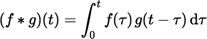
The ∗ operator is associative and commutative. Associativity implies that if we have functions f1(t), f2(t), …, fn(t), we can write (f1 ∗ f2 ∗ ⋯ ∗ fn)(t) without ambiguity. Commutativity implies that (f ∗ g)(t) = (g ∗ f)(t).
Note: The definition implies that (f ∗ g)(0) = 0. In fact the first n − 2 derivatives of a convolution (f1 ∗ f2 ∗ ⋯ ∗ fn)(t) are also zero at t = 0.
An atom initially in state S1 will be in state Sn after time t has elapsed iff (if and only if) it decays through the first n − 1 states before time t and then remains in state Sn till time t without decaying further. So, the event En occurs iff T1 + T2 + ⋯ + Tn − 1 ≤ t and Tn > t − (T1 + T2 + ⋯ + Tn − 1). So, the atom ingrowth factor IFatom is equal to the probability Pr[En], given by:

Notice that if Sn is stable, then λn is zero and IFactivity = 0, but IFatom ≠ 0 unless the ingrowth time is zero.
In order to calculate either of these factors, one needs to be able to calculate the convolution of the exponential functions Dλ1(t), Dλ2(t), …, Dλn(t). The theoretical solution to this problem is well known. The difficulties arise when one tries to implement the algorithm efficiently for a computer in a manner that avoids severe floating-point cancellation errors.
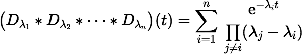
If all the decay constants are distinct (the usual case in the real world), the convolution is given explicitly by:
 |
(∗) |
which is easily coded in a programming language like C, C++, C#, Java, or Fortran. (For the case where some of the λi are repeated, see below.) Equation (∗) may look familiar to those who have dealt with the ingrowth problem before.
Note: The value of the convolution is zero at t = 0, as mentioned above, although this fact may not be immediately obvious from Equation (∗). The function’s first n − 2 derivatives are also zero at t = 0.


Rounding Error
Consider the simplest nontrivial example, where n = 2. In this case Equation (∗) simplifies to the following:

This convolution can be used when calculating the ingrowth of an immediate daughter product from a parent. Even in this simple example there is the possibility of large rounding error. Suppose t is very small. In this case the numerator evaluates to the difference between two numbers that are nearly equal to 1. The most straightforward implementation of the equation in a computer language will lead to an unnecessary loss of accuracy, possibly even returning zero in situations where the true value, although it may be small, is well within the machine’s range of positive floating-point values.
An obvious fix in this simple case when t is small is
to use the Maclaurin series for the convolution (see below).
However, there is an even easier fix in any programming language that has a library function for the
hyperbolic sine (sinh).

where λ = (λ1 + λ2) / 2, and b = (λ2 − λ1) / 2.
Warning: Do not use this trick in older versions of Microsoft Excel. My 2007 version of Excel uses a naïve implementation of
sinh. It calculates
sinh with the following equation, which fails for extremely small values of the argument:

The C language and some implementations of its derivatives also
provide a library function expm1(x), which calculates
ex − 1
accurately. The convolution equation can be written using expm1 as follows:

where d = λ2 − λ1.
If you have the expm1 function in your library, you should use it here.
For many of the most common ingrowth examples in the radiochemistry lab, either of the two preceding equations will suffice. If there were no more complicated situations than this, the problem would be completely solved; however, there are more complicated examples where n > 2. For instance one may want to calculate the ingrowth factor for a descendant of a very long-lived radionuclide, where some of the intermediate states are long-lived and some are short-lived. This is another situation that can lead to severe round-off error. (E.g., try calculating 1 year’s worth of 222Rn ingrowth from 238U.)
Equation (∗) has the potential to produce excessive round-off error whenever there is a cluster of distinct values λi t that are too close together. This can happen when the values are large, but it is more common when they are small, as in the simple (n = 2) example described above when t is small, or in the 238U example, where several of the half-lives are very long. Whenever λi t and λj t are small and almost equal—but not quite—Equation (∗) has large positive and negative terms that almost cancel each other—but not quite. The rounding error in this case may be larger than the actual value.
The Maclaurin Series
When t is small enough, the Maclaurin series for the convolution gives fast and accurate results. This series can be written as follows:

where (n)k is the Pochhammer symbol, or the rising factorial, (n)k = (n)(n + 1)(n + 2)…(n + k − 1), and where hk(x1, x2, …, xn) denotes the complete homogeneous symmetric polynomial of degree k, in n variables, defined by:

The rising factorial is easy to evaluate incrementally for successive values of k, because (n)k + 1 = (n)k (n + k). Fortunately hk(x1, x2, …, xn) is also easy to evaluate incrementally.
- h0(x1, x2, …, xn) = 1
- hk + 1(x1) = x1k+1 = x1 hk(x1)
- hk + 1(x1, x2, …, xi+1) = hk + 1(x1, x2, …, xi) + xi + 1 hk(x1, x2, …, xi + 1)
So, the Maclaurin series is easy to code. It also has the virtue of converging for all values of t, but the convergence is rapid enough to be practical for computation only if all the λi t are somewhat smaller than 1. There are many possible scenarios where some of the λi t are too large to give rapid convergence of the Maclaurin series while others are so small (and therefore close together) that they lead to unacceptable round-off error in Equation (∗).
When all the λi t are small enough, the convolution is approximated well by the first one or two nonzero terms of the Maclaurin series.

The (atom) ingrowth factor is then approximated by:

An example of a scenario where this approximation is useful is the calculation of ingrowth in the decay chain 234U → 230Th → 226Ra, where all three half-lives are fairly long. Using Equation (∗) as written, with ordinary double-precision arithmetic, to calculate the ingrowth of 226Ra over a time interval shorter than a year is likely to produce a larger rounding error than using just the first two terms of the Maclaurin series.
Note: By comparing the coefficients in the Maclaurin series above with the derivatives of Equation (∗) evaluated at t = 0, one finds that:

If all the λi t are approximately equal but none is small, the following identity allows one to compute the convolution rapidly using a Maclaurin series (e.g., with c = λ).

However, such a situation is unlikely to arise in practice. So, it seems that the most obvious approach to the problem of round-off error won’t completely solve it.
The Laplace Transform
Before exploring other options, it will help to introduce a powerful tool for dealing with the problem: the Laplace transform. If f (t) is a function of a non-negative real variable t, the Laplace transform of f (t) is the function F(s) defined by:

where s and F(s) are generally considered to be complex.
If F(s) is the Laplace transform of a function f (t), as shown above, and if F(s) is meromorphic with poles c1, c2, …, cn, which may be either real or complex, then its inverse Laplace transform is:

where Ress = ci{est F(s)} means the residue of est F(s) at the pole ci.
Many useful facts about the function f (t) = (Dλ1 ∗ Dλ2 ∗ ⋯ ∗ Dλn)(t) can be derived by algebraic manipulation of the transformed function F(s) followed by application of the inverse transform. Although the same facts can be derived in other ways, the derivations using the Laplace transform tend to be easier.
Instead of applying the equations shown above for the Laplace transform and its inverse, it usually helps to remember some common functions and their transforms—or have access to a table of these—and to remember that both the transform and its inverse are linear.

The Laplace transform of an exponential function Dλ(t) = e−λt is particularly simple:

By setting λ = 0, we see that:

The Laplace transform of a convolution (as defined above) is just the product of the transforms of the individual functions.

where F(s) and G(s) are the Laplace transforms of f (t) and g(t), respectively. So, the Laplace transform of our convolution is the rational function:

Applying the Laplace Transform
The transformed function can be manipulated algebraically to produce new expressions for the original convolution, and some of these new expressions lead to algorithms for computation with less round-off error. Sometimes the new expression is an infinite series, each term of which involves a convolution of exponential functions where each λi from a problematic cluster has been replaced by a single value μ, which might be one of the original λi from the cluster or perhaps the cluster average. Substituting a single value μ for several of the λi produces a convolution in which the decay constants are not all distinct and to which Equation (∗) doesn’t apply.
So, now we need the more general form of Equation (∗), which doesn’t require all the decay constants to be distinct. For lack of a better notation, define Gμ, n(t) to be the n-fold convolution of the single exponential function Dμ(t).*

The Laplace transform of Gμ, n(t) is:

Our next goal is to derive expressions that can be used to calculate the function g(t) defined by:

where each mi is a positive integer. The Laplace transform of g(t) is:

The function G(s) is meromorphic, because it is a rational function. In general, if F(s) is the Laplace transform of a function f (t) and F(s) is meromorphic with (real or complex) poles c1, c2, …, cn of orders m1, m2, …, mn, respectively, then:

In our problem the function G(s) has poles −μ1, −μ2, …, −μn. So,

where Ai, k is given by:

The expression for Ai, k doesn’t look very useful for computation, but with a little work one gets the following:

where the bullet notation m • x indicates that an argument x is repeated m times in the argument list. With another abuse of notation, we can rewrite the preceding equation as:

Then we can write the more general form of Equation (∗):

|
(∗∗) |
Of course Equation (∗∗) has the same round-off issues as Equation (∗) when the μi t are clustered together, but it works well enough when the μi t are well separated, and unlike the Maclaurin series, it doesn’t have slow convergence (and is less likely to overflow) when the μi t are large.
Note: The fact that g(0) = 0 implies:

Other Series
Some relevant facts about the complete homogeneous polynomials:

where each ki ≥ 0 and each zi ∈ ℂ.

where σ is any permutation of the set {1, 2, …, n}.
 , for
∥ z ∥ <
1
, for
∥ z ∥ <
1
 , if each
∥ zi ∥ <
1
, if each
∥ zi ∥ <
1
 , if each
∥ zi ∥ <
1
, if each
∥ zi ∥ <
1


Using these facts we can easily derive the Maclaurin series for f (t).


With a few changes we can derive other series. Suppose for each λi we choose a μi, which may or may not be equal to λi. Then F(s) can be rewritten as follows:

where the ki are non-negative. Then:
 |
(∗∗∗) |
This series is essentially a multivariable Taylor series in the variables λ1, λ2, …, λn. It can be made useful for calculation if we choose the μi carefully. For rapid convergence the differences | μi t − λi t | must be small (at least smaller than 1). The series will be simpler if there is only one or at most a few distinct μi for which μi ≠ λi, but the number of the μi needed to keep the round-off error small is really determined by the number of λi clusters, because the μi must be well separated. If there is only one cluster, the resulting series will be simple enough. Say the λi are arranged in increasing order, and the first r of them form a cluster. We can let:

and μi = λi for i > r. Then write f (t) as follows:
 |
(∗∗∗∗) |
If there is more than one cluster of decay constants λi, then a more complicated series is needed, but in many situations Equation (∗∗∗∗) suffices.
Given that μ = (λ1 + λ2 + ⋯ + λr) / r, it is important to note that the second term of this series (k = 1) is zero. So, convergence cannot be tested until k ≥ 2.
Implementing the series efficiently requires an efficient algorithm for updating (Gμ, r + k ∗ Dλr + 1 ∗ ⋯ ∗ Dλn)(t) for successive values of k. If λr + 1, λr + 2, …, λn are distinct, then:

where:
 and
and  , for
i = r + 1, r + 2, …, n,
, for
i = r + 1, r + 2, …, n,
and where for any N and any x1, x2, …, xp,

Notice that W does not depend on k; so, it is calculated only once. Also notice that:

The algorithm can employ a simple vector to hold the values of Cr + 1, k , Cr + 2, k , …, Cn, k and after each Ci, k is used, replace it with Ci, k + 1. Most of the work of incrementing k is done in the recalculation of φr + k − 1, but there is an incremental algorithm for this calculation, and its complexity remains constant as k increases. Define:

Then φ0(t; x1, x2, …, xp) = 1. For N ≥ 0,

and for i = 1, 2, …, p,

So, the time required to recalculate φN(t; x1, x2, …, xp) for each new value of N is proportional to p but not to N.
The Siewers Algorithm
I discovered the Siewers algorithm—fortunately or unfortunately—only after doing a lot of work on the problem myself. This algorithm is based on the fact that:
 , for
λi ≠ λj,
, for
λi ≠ λj,
where the check over a symbol (Ď) indicates a function omitted from the convolution. I actually knew this identity already but had not noticed that it could be used to develop an efficient algorithm. At first glance it appears to be O(2n), but it can be implemented more efficiently than that.
Define:

Then:

So, if we can calculate the function F reliably, we have solved our original problem too.
Notice that the value of F(x1, x2, …, xn) does not depend on the order of the arguments. So, rearrange the arguments if necessary to ensure x1 ≤ x2 ≤ ⋯ ≤ xn. The Siewers algorithm now calculates F(x1, x2, …, xn) using the recursion:
 |
(∗∗∗∗∗) |
if the difference xn − x1 is large enough (greater than some value δ). If the difference is too small, then:

where c = (x1 + xn) / 2, and where the Maclaurin series is used for F(x1 − c, x2 − c, …, xn − c).
Very small values of δ ensure rapid and accurate conversion of the Maclaurin series, while larger values tend to minimize round-off error in the recursive calculation (∗∗∗∗∗). The most appropriate choice of δ balances these two considerations. A value between 1 and 2 is likely to give acceptable results. (I get slightly better accuracy with 2 than with 1.)
The only remaining issue is how to avoid unnecessary recalculation of intermediate quantities of the form F(xi, xi + 1, …, xj) that are needed more than once by the algorithm. For s = 1 to n − 1, and for i = 1 to n + 1 − s, if either xi + s − xi > δ or xi + s − 1 − xi − 1 > δ, then calculate:

using the most appropriate method. If s = 1, then of course the most appropriate method is given by:

If s > 1, and if xi + s − 1 − xi > δ, then:

Otherwise, calculate:

where c = (xi + xi + s − 1) / 2, using the Maclaurin series.
Finally, calculate and output f1(n), which equals F(x1, x2, …, xn).
In fact, a single array of length n can be used to hold the values fi(s) at each step of the iteration (s = 1 to n). The algorithm calculates the following quantities as necessary:
| i = 1 | i = 2 | … | i = n − 1 | i = n | |
| s = 1 | f1(1) = F(x1) | f2(1) = F(x2) | … | fn−1(1) = F(xn−1) | fn(1) = F(xn) |
| s = 2 | f1(2) = F(x1, x2) | f2(2) = F(x2, x3) | … | fn−1(2) = F(xn−1, xn) | |
| ⋮ | ⋮ | ⋮ | ⋰ | ||
| s = n − 1 | f1(n − 1) = F(x1, x2, …, xn − 1) | f2(n − 1) = F(x2, x3, …, xn) | |||
| s = n | f1(n) = F(x1, x2, …, xn) | ||||
The quantities in each row after the first are calculated either (a) recursively, using two of the quantities from the preceding row or (b) using the Maclaurin series. The last row holds the final result.
Final Note
Recall Equation (∗∗∗):
This equation would be most useful if we had an efficient incremental algorithm to calculate the sum:

for increasing values of k. An incremental algorithm is easy enough to find—it’s making it efficient that’s hard. (Earlier we obtained efficiency with the assumption that there was only one distinct value of μi for which μi ≠ λi.) There is a simple incremental algorithm to calculate:

and in fact there is a very efficient incremental algorithm to calculate:

which follows from the somewhat unexpected fact that:

Recalculating this sum when incrementing k requires only a multiplication by t and a division by the new value of k.

Although this sum is easy to calculate, we unfortunately have no need for it. There may be a simple and efficient algorithm for the sum we do need, but this programmer doesn’t know it yet.
The Siewers algorithm looks best.
Algorithms: A few explicit algorithms for some of the calculations described above
Example: 238U → 222Rn — to be completed
Application to mean decay or ingrowth during counting — not completed, but simple (include D0(t) ≡ 1 in the convolution and divide the final result by t)
Uncertainty of a decay or ingrowth factor — to be completed (theoretical value obtained by propagating uncertainties of time and decay constants would be misleading in the presence of large and unknown rounding error)
See also Non-Poisson
Counting
 — The derivation of equations for the index of dispersion (
J factor
) in non-Poisson counting measurements
makes use of ingrowth
factors for short-lived decay products (e.g., 222Rn
progeny). For a PowerPoint summary see Non-Poisson Counting Statistics, or
What’s This J Factor All About?
.